Recent advances in solid state physics have led to the discovery of fundamental relationships between charge currents and spin currents. These relationships are due to the spin-orbit moments of electrons. Among these effects are the Spin Hall Effect—the accumulation of spins due to a charge current—and the Inverse Spin Hall Effect. The most popular characterization experiment utilizes Ferromagnetic Resonance to generate and pump a spin current into a non-magnetic material, resulting in a measurable voltage due to the Inverse Spin Hall Effect. This data is then used to develop a macroscopic model to analyze experimental phenomena—how the delivered power decays from the signal generator to the sample. Developing a granular microscopic model will allow for analysis of what occurs within the sample material itself, for various experimental conditions.
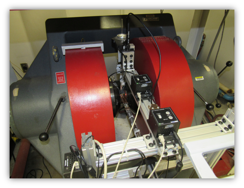
The common method--and the method we ascribe to--for generating a spin current is to use a Ferromagnetic Resonance (FMR) machine. This machine uses two high power electromagnets to unifromly magnetize a material. Then, it uses a microwave generator to apply a high frequency magnetic field that forces the internal magnetic moment of the material to rotate about the applied external field. The process of this rotation generates a spin current, as the electron magnetic moments are aligned with the external field, and move upward as a spin curent into the nonmagnetic layer of the test sample.
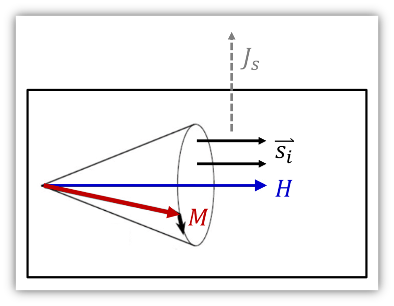
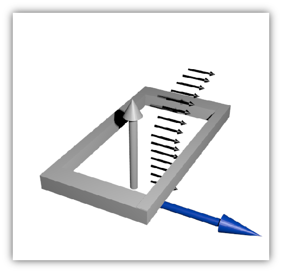
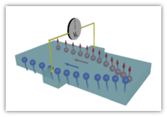
The upward motion of the electrons form the upward spin current Js flows into the nonmagnetic material layer, pictured below. Once it enters into the nonmagnetic layer, it generates a charge current due to the Inverse Spin Hall Effect. This charge can be described with \[Jc = D_{ishe} (\vec{J_s} \times \vec{\sigma}) \] In the above equation, \(\vec{D_{ishe}}\) represents the ISHE efficiency, and \(\vec{\sigma}\) represents the spin polarization vector (the direction of the electron's spin magnetic moment). The image below (left) depicts what happens when electrons move into the nonmagnetic layer--they deflect to one side, building up and creating a voltage accross the material.
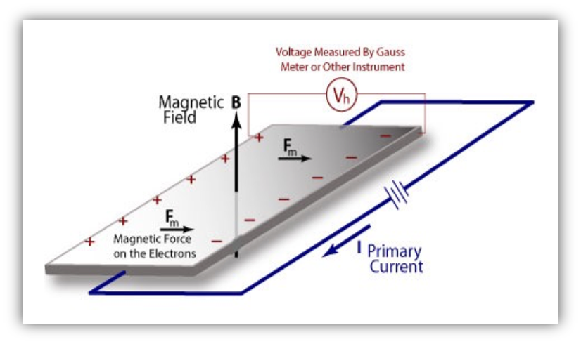
The image on the right (above) depicts how the Spin Hall Effect and Inverse Spin Hall Effect are analogous to, and best understood in, the context of the classical Hall Effect. When a current-carrying wire is placed in an external magnetic field, the electrons experience the force: \[\vec{F} = e(\vec{v} \times /vec{H})\] which generates the derived voltage \(V = \dfrac{IB}{ned}\).
However, electrons possess two intrinsic magnetic moments: the orbital magnetic moment (which contributes to the Anomalous Hall Effect) and the Spin Hall Effect, which produces the Spin Hall Effect. Electrons with opposing spins deflect in opposite directions, creating a symmetric spin current as all the electrons moving in a given direction have the same magnetic moment. So we can use an external magnetic field to generate a spin current, and that spin current will in turn generate a charge current.
We used an FMR machine to generate a spin current, which in turn produced a transverse charge current in the nonmagnetic layer. This diffusion formed a measurable voltage across the material. This voltage was measured experimentally (linked to the oscillating behavior of the FMR machine), but we also analyzed it theoretically using the following two equations: \[V_{ishe} = \dfrac{-\gamma g_{\updownarrow} eL \lambda_{sd} \omega}{2 \pi \sigma_N t_N}sin(\alpha)sin^2(\theta)tanh(\dfrac{t_N}{2\lambda_{sd}})\] \[\theta = \dfrac{h_{rf}cos(\alpha)}{\Delta H sqrt{1 + ( \dfrac{(H_{dc}-H_r)(H_{dc}+H_r+4\pi Ms)}{\Delta H 4 \pi M_s})^2 }}\]
These equations were used to develop a computer simulation to model the experiment. After running an experiment (with the help of Dr. Jamileh Beik Mohammadi, who was a grad student at the time) I wrote Matlab software which would import the FMR and Voltage data for a material, then compile this data and automatically extract certain important magnetic parameters (e.g. \(\gamma, \Delta H, V_{max}, M_s\)). The simulation then uses this data to compute \(V_{ishe}\) over the range of experimentally acquired values.
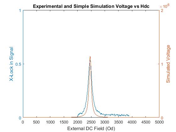
During testing, we select a specified input frequency for energizing the magnetic material, then perform a DC field sweep to find the point at which we recieve maximum resonance in the Ferromagnetic layer (i.e. ferromagnetic resonance). The graph below contains the data obtained from measuring the voltage for each of these tests, overlayed with the simulation's output for each of the corresponding frequencies.
The main advantage for developing a simulation like this one is that it allows a researcher or designer to rapidly test how a material might behave in certain conditions. In line with this goal,
this simulation allows for testing independent of the data; i.e. any frequency can be tested. This allows for higher resolution tests.
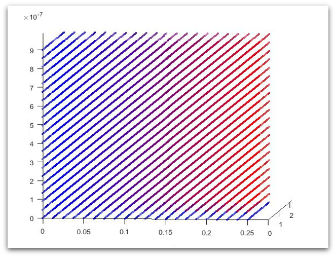
Pictured below is a suite of simulated values vs External field.

In an attempt to gain a greater understanding of the behavior within the nonmagnetic layer, I begain developing an abstraction of the simulation that would model the magnetic moments within the material itself. This simulation still requires further development, so it is difficult to see how the magnetic moments accumulate on one side of the material (depicted as red vectors on plot below).